User Area > Advice
Equivalent force distribution
In the finite element method, the
equilibrium equation {f}=[K]{d} is solved for displacements {d} at the nodal locations.
Hence, both the applied forces {f} and the stiffness {K} are required at these nodal
positions. For example, the assignment of a constant body force (force per unit volume)
requires that a transformation be performed from the volume-based loading to a set of
equivalent concentrated loads that are then applied to the nodes – hence the force
vector is commonly termed the equivalent nodal load vector.
Such force vectors are also termed
“consistent” because the same assumptions (shape functions, integration order
etc.) are used as in the generation of the stiffness matrix. That is, the stiffness and
the force are consistent with each other. The only exceptions to this are the continuum
solid elements and section 5.1 of the theory manual (“General Load Types”)
should be consulted for further information
This section describes the way in which the
finite element assumptions are used to convert a force on an element into equivalent nodal
loading, specifically, the application of a uniformly distributed load to a 3-noded bar
element.
The equivalent nodal force load {r} for
such a uniformly distributed loading {p} is given by
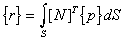
Where [N] are the shape functions and S is
the area over which the uniformly distributed load integration is to be performed.
In the case of a 3-noded bar element, the
axial distributed load {p} is applied as follows
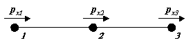
and in vector form as

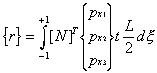
If t
is the width of the bar and dx, an incremental
length along the bar, then the incremental surface area is

Given

So that

Therefore,
changing the integration limits from the local to the natural
coordinate system, the equivalent nodal force is given
by
Using the quadratic shape function for this bar element
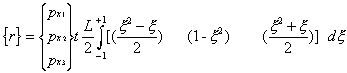
This integral
is accurately evaluated using a two-point Gauss
integration rule in which the weight is 1 and the optimum
sampling points are  .
So that .
So that
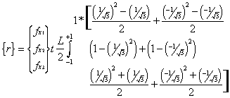
Or finally
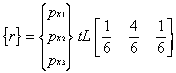
Thus a constant, uniformly distributed load
applied along the length of a 3-noded bar element is transformed into equivalent nodal
loads which are distributed according to the ratio  .
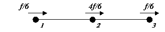
If the equivalent nodal forces (px1*tL),
(px2*tL) and (px3*tL) are denoted by the constant f, then,
diagrammatically this distribution becomes .
If the equivalent nodal forces (px1*tL),
(px2*tL) and (px3*tL) are denoted by the constant f, then,
diagrammatically this distribution becomes
The same distribution is obtained for
uniformly distributed edge loading on an 8-noded, 2D plane element of side length (L) and
thickness (t), as follows
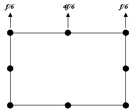
A constant, uniformly distributed load {p}
applied to the surface of an 8-noded surface element can be similarly examined to observe
the ratio of the corner and midside nodes to be  ,
diagrammatically shown as follows ,
diagrammatically shown as follows
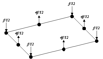
In this case, f = A*p,
where (A) is the surface area of the
element.
Because the element stiffness and forces
are consistent with each other, this apparently “incorrect” distribution is
actually entirely valid and, indeed, essential.
A number of implications arise from the use
of the equivalent load vector in finite element analyses and are considered below.
Implication: Equivalent Loading Across Multiple Elements
The foregoing discussion has been
based on a higher order element. The use of lower order elements does not produce such an
anomaly and the load is distributed equally between the nodes of the element.
When elements are combined in a mesh
and loading applied across multiple higher order elements the same distribution takes
place. It is worth noting, however, that the nodes common to the adjoining elements
receive a force contribution from each of these elements. As an example, consider the
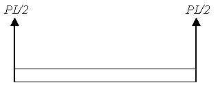
diagram below in which two, higher order elements are subject to a constant, uniformly
distributed load (p), as before.
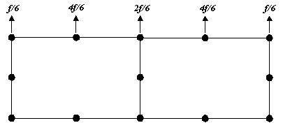
In this case the centre node receives an
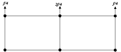
equivalent force contribution from the two adjoining elements of (2f*1/6)). The same is true for a linear element assemblage
as follows
If a summation of element reactions is
performed over a single element then this additional contribution from the adjacent
element(s) would need to be subtracted to be absolutely correct.
Implication: Loading Attribute Visualisation Arrows In Reverse
Directions
With a model load case active, select the
attribute properties and then the loading tab. Press the button marked
“settings…”, where the following two options will be seen
- “Show discrete loading by
definition”
- “Show discrete loading by
effect on mesh”
By default the latter is invoked and will
show the equivalent nodal forces as described above, whilst the former will visualise the
forces as defined in the attribute definition without any additional transformation into
equivalent loads. This explains why visualising the loading attributes on a mesh, can
produce a series of arrows that either alternate unexpectedly in size or reverse in
direction.
Discrete loads are not the only loading
types that are processed in this way for higher order elements; it applies equally to
practically all loading types.
Implication: Planar Displacement Fields
Applying “Concentrated Loads” to
the edge of a higher order element to produce a uniform and planar displacement of all the
nodes on that edge requires that the concentrated loads be applied in the ratios given
above.
The “Global Distributed” loading
also applies concentrated loads directly to the nodes in the same way that selecting the
“Concentrated” load tab would, however, in the former case, the element shape
functions are accounted for and the distribution handled automatically.
All other loads in LUSAS are also handled
automatically.
Implication: Reactions Are Unexpectedly Not Constant Along A
Supported Boundary
Support reactions are also distributed
according to the same principles. Hence the constant nodal reactions that would be
naturally expected from the application of a uniformly distributed load would actually be
distributed in the ratios given above.
The sum of the reactions over a single
element, however, will accurately represent the total reaction acting over the length/area
of the element.
Implication: Equivalent Nodal Loading For Beam/Shell/Plate
Elements
This equivalent nodal load transformation
(or decomposition) must produce kinematically equivalent nodal forces from the applied
element loads for elements that support moment output. For such elements, this will mean
that a constant uniformly distributed load over the length of the element will produce
both an equivalent shear force and a bending moment.
Kinematically equivalent loads are so named because they replace
a distributed load so that the correct work is maintained. To replace the distributed load
by statically equivalent forces would be
incorrect and could result in errors when solving for the displacements – especially
in coarse mesh definitions.
In MODELLER, kinematically equivalent loads
are calculated for the relevant elements automatically.
For example, a constant value of uniformly
distributed load (P) on a single beam element of length L has a kinematically equivalent
nodal load defined as follows
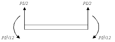
Whereas, the statically equivalent load is
defined as follows
It is for this reason that visualisation of
loads in MODELLER can display additional moments at nodes on which a uniformly distributed
load has been applied.
Discrete loading is an important exception
to this general rule of decomposition. Discrete loading is applied to the finite element
mesh and is converted into equivalent nodal loads using the shape functions of the
elements. These nodal loads are then applied directly to the underlying structural mesh.
Although these nodal loads correctly represent the vertical and in-plane components of the
applied loading, they do not account for any kinematic decomposition. The effect of this
is mesh dependent and, in the general case, is not an issue. For very coarse meshes this
assumption may cause the results to be affected.
Implication: Joining Lower And Higher Order Elements
It is tempting on occasion to try to
join lower and higher order elements together, typically when attempting to generate a
mesh transition from higher order elements to low order element. For instance, consider
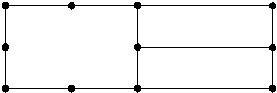
transitioning from 4-noded to 8-noded quadrilateral elements as follows
To demonstrate the effect of mixing
elements in such a manner, consider the above situation in which a prescribed displacement
of unity is applied to one end of the structure with support conditions as follows
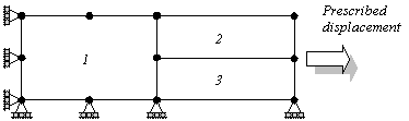
This loading is expected to produce a
planar response throughout the structure as shown in the top-most diagram (below) where
two 8-noded quadrilaterals are used. The lower of these two diagrams is the response when
mixing the element types. Both diagrams show the nodal displacement magnitudes in the
X-direction.
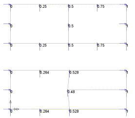
The reason for the non-planar displacement
field obtained may be seen by considering the equivalent nodal force distributions
required for both the 4-noded and 8-noded elements to transmit such a planar force. The
following diagram shows the distributions at the element interface
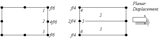
For the expected results to be obtained the
distribution needs to be identical. If the difference in the distribution ratios is
considered we have
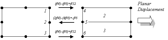
Although the total force across the
interface will be correct, the distribution of the force will not be. That is, the
difference in the ratio at nodes 1 and 4 produce a net difference in the loading of f/12,
whereas nodes 2 and 5 produce a net difference of f/6 in the opposite direction. The
direction of these force ratio differences correlate with the non-planar displacements
that are seen, that is nodes 1 and 4 displace in the same direction as the net f/12 force
and nodes 2 and 5 displace according to the direction of the f/6 net force.
If it is necessary to join elements in such a manner, it is
recommended that constraint equations be used to ensure that the nodes along the element
interface are constrained to displace in a planar manner.
In summary, the joining of low and
high order elements in such a manner is a dubious practice, to be avoided if at all
possible and is discouraged on the basis of the different nodal force distribution (as
well as stiffness) associated with the different element types which may cause inaccuracy
in the results. Together with this inaccuracy the possibility of exciting an element mechanism in the 8-noded element when reduced
integration is being used is greatly increased.
Finite
Element Theory Contents
Local
Coordinate System
Shape
Functions
Numerical
Integration
|